Hello there,
With first evaluations passed (thanks, mentors), and after more time than the ideal, I return to finish our FMI2-wrapper computational function.
Exchanging some e-mails and revisiting available documentation (FMI specification is too long to get by looking at it a single time) made me realize that my previous code was quite incomplete. As I fixed it, I have also updated the related blog reports (here, here and here), keeping this one just for new additions and information.
Implicit vs Explicit
As it turns out, current Scilab implementation treats Modelica blocks always as implicit (DAE based), so that the simulator solver is changed to IDA type every time it contains this kind of block. That way, our derivatives calculation stage actually will always have to return residual values rather than state time derivatives themselves.
In Scicos blocks case, when dealing with DAE solvers, the main simulator has to be informed about the nature (differential or algebraic) of each state variable. This is defined through xprop block field, during calls to the computational function with flag 7.
/* ... */

void fmi2_block( scicos_block* block, const int flag )
{
    switch (flag)
    {
        /* ... */

        // Flag 7: Define property of continuous time states (algebraic or differential states)
        case ContinuousPropertiesUpdate:
        {
            for( int i = 0; i < block->nx; i++ )
                block->xprop[ i ] = /* 1 for differential state, -1 for algebraic one*/;

            break;
        }

        /* ... */
    }
}
However, the way a Model Exchange type FMU model libray handles DAEs is such that one can’t transparently expose this information. As stated in the documentation:
- The FMI for Model Exchange is for ordinary differential equations in state space form (ODE). It is not for a general differential-algebraic equation system. However, algebraic equation systems inside the FMU are supported (for example the FMU can report to the environment to re-run the current step with a smaller step size since a solution could not be found for an algebraic equation system).
Basically, algebraic states aren’t exposed to the host application, instead, algebraic restrictions would be used to trigger state changes handle internally, while only differential values compose the states array. That way, our block is presented to the simulator as a ODE, with all xprop values equal to 1.
Entering the [Jacobian] Matrix
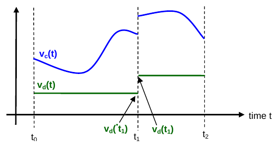
Even if a FMU model represents a time continuous system, things like inputs and other events are applied in discrete steps, causing discontinuities:

(Piecewise-continuous variables of an FMU: continuous/hybrid variables in blue (vc))
To handle those jumps recalculating model state, computational functions are called with flag 10, asking for a matrix of states and outputs partial derivatives, that compose the system’s Jacobian matrix, used by KINSOL nonlinearity solver.
In practice, here the partial derivatives are discrete, representing how much system’s functions (xd=f(u,x,t)) and outputs (y=g(u,x,t)) change from a particular situation, for a small change in each state variable:
(Partial derivatives matrix for system with 2 states [derivatives] and 2 outputs. Made with CodeCogs)
And here is the code that was left out of my last post (shame on me !):
/* ... */

SCICOS_IMPEXP void BLOCK_FUNCTION_NAME( scicos_block* block, const int flag )
{
   switch (flag)
   {
      /* ... */

      // Flag 10: Jacobian computation
      case Jacobian:
      {
          fmi2Real dx = 1.0;      // State variation for discrete derivatives calculation

          // Define input and state for which the derivatives are calcuated
          fmi2SetTime( (fmi2Component) block->work, get_scicos_time() );

          set_input( block );

          fmi2SetContinuousStates( (fmi2Component) block->work, block->x, block->nx );

          for( int i = 0; i < block->nx; i++ )
          {
              fmi2GetDirectionalDerivative( (fmi2Component) block->work,
                                            STATE_REFS_LIST + i, 1,          // array and number of derivated state references
                                            STATE_DER_REFS_LIST, block->nx,  // array and number of derivative references
                                            &dx, stateDerivativesList );     // state deltas and resulting state derivatives

              // Fill matrix column top with acquired values
              for( int i = 0; i < block->nx; i++ )
                  block->res[ i * block->nx ] = stateDerivativesList[ i ];

              fmi2GetDirectionalDerivative( (fmi2Component) block->work,
                                            STATE_REFS_LIST + i, 1,         // array and number of derivated state references
                                            OUTPUT_REFS_LIST, block->nout,  // array and number of output references
                                            &dx, outputsList );             // state deltas and resulting output derivatives

              // Fill matrix column bottom with acquired values
              int xd_mat_size = block->nx * block->nx;
              for( int i = 0; i < block->nx; i++ )
                  block->res[ xd_mat_size + i * block->nx ] = outputsList[ i ];
          }

          break;
      }

      /* ... */
   }
}
Wrapping up
That almost concludes what is needed for our C computational function. The only thing missing is a way to store in the block the input and output variables references (indexes). That would involve taking this information from the model description XML file (my next goal, btw), as those values are not always located in the same positions of the real variables list (like states and derivatives).
Thanks for sticking with me one more time. See Ya !